OLAP vs. OLTP: The Difference Between Analytics Databases and Transaction Systems

OLTP (online transaction processing) databases handle the small, fast reads and writes an application makes: place an order, update a balance, load a profile. OLAP (online analytical processing) databases answer questions across millions of rows at once: revenue by country this quarter, churn by signup month. Postgres and MySQL are OLTP systems. BigQuery, Snowflake, Redshift, and ClickHouse are OLAP systems.

The standard production pattern runs both, with a pipeline copying data from the transactional database into the warehouse. This article covers why the two are built so differently, what that does to your bill, and how the copy from one to the other works.

What is the difference between OLAP and OLTP?

OLTP processes transactions: many small reads and writes that each touch one or a few rows and finish in milliseconds. OLAP analyzes data: few large queries that each read millions of rows and finish in seconds or minutes. The primary purpose of OLAP is to analyze aggregated data, while the primary purpose of OLTP is to process database transactions.

The two terms come from different eras. Transaction processing is as old as databases. The term OLAP was coined in 1993 by Edgar F. Codd and colleagues, the same Codd who defined the relational model. An OLTP operation touches tens or hundreds of records at most, while an OLAP query touches thousands or millions.

Here is what each side looks like in SQL. A typical OLTP query fetches one customer's latest orders:

SELECT order_id, order_value, created_at
FROM orders
WHERE customer_id = 7842931
ORDER BY created_at DESC
LIMIT 5;

With an index on customer_id, Postgres answers this in a few milliseconds even on a billion-row table, because it reads one index path and a handful of pages.

A typical OLAP query totals revenue by country for the quarter:

SELECT country, sum(order_value) AS revenue
FROM orders
WHERE created_at >= '2026-02-01'
GROUP BY country
ORDER BY revenue DESC;

A columnar engine reads only the country, order_value, and created_at column files, skips the date ranges outside the filter, and sums in batches. A row store has to read the full row for every order in the quarter, which is far more disk work for the same answer.

What workloads belong in an OLTP database and an OLAP warehouse?

Anything a user is waiting on belongs in OLTP. Anything that summarizes history belongs in OLAP. For a retail business, the OLTP side processes sales, inventory changes, account updates, loyalty points, payments, and returns. The OLAP side analyzes sales trends, inventory levels, customer demographics, and historical patterns over the same data.

Two standard benchmarks show the split clearly. TPC-C is the standard OLTP benchmark. It runs a mix of five concurrent transaction types (new order, payment, delivery, and so on) and scores in transactions per minute. TPC-H is the standard decision-support benchmark. It runs complex queries over large data volumes and scores in queries per hour at a given data size. One measures how many small things you can do per minute. The other measures how many big questions you can answer per hour.

The write side differs just as much. An OLTP system sees a steady stream of single-row inserts and updates. An OLAP system takes bulk inserts and is append-mostly. Snowflake supports single-row updates, but an update rewrites the entire 50 to 500 MB micro-partition that holds the row. That is fine for a nightly load and unworkable for thousands of small writes per second.

Why are OLAP databases column-oriented while OLTP databases are row-oriented?

A row store keeps all the fields of one record together on disk, which is what you want when you read or update one whole record. A column store keeps all the values of one column together, which is what you want when you sum one column across millions of records. Each layout is fast at what the other is slow at.

In a row store, loading a user profile is one read of one contiguous chunk. In a column store, the same operation touches every column file, and inserting one row does too. The column layout can take in millions of rows per second in bulk but handles single-row changes poorly.

The column layout has a second benefit: compression. When values of the same type and often the same value sit next to each other, compression algorithms find long repeated patterns. ClickHouse's Stack Overflow example table compresses 143.47 GiB down to 50.16 GiB overall, a ratio of 2.86. One low-variety column in that dataset, CommentCount, went from 56.84 MiB to 635.78 KiB, a ratio of 91.55. Per-column results vary a lot with the data type, sort order, and codec, so those numbers describe that table, and yours will differ.

Less data on disk means less data to read per query. Combined with only reading the columns a query names, this is why a warehouse can answer the revenue-by-country query above without touching most of the table.

How do partitioning and clustering reduce warehouse scans and cost?

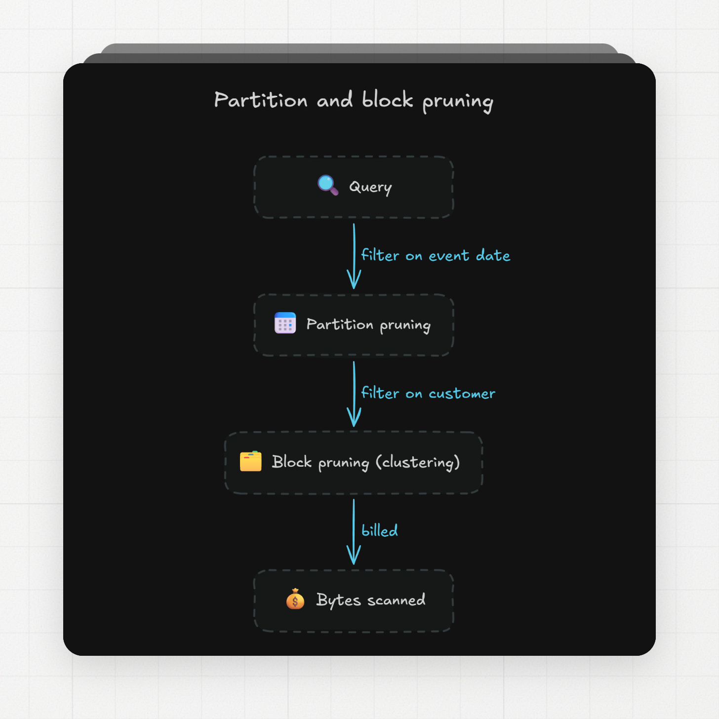
Partitioning splits a table into segments by one column (usually a date), so a query that filters on that column reads only the matching segments. Clustering sorts the data inside those segments by a few more columns, so the engine can skip blocks that cannot contain matching rows. Both cut the bytes a query reads, and on a pay-per-scan warehouse, bytes read is the bill.

In BigQuery, a partitioned table is divided into segments called partitions. If a query has a qualifying filter on the partitioning column, BigQuery scans the partitions that match and skips the rest. A table can be partitioned by one column only, and partitioning fits best when each partition holds under about 10 GB.

Clustering picks up from there. A clustered table has a user-defined sort order on up to four columns. BigQuery stores data in blocks sorted by those columns, and when a query filters on them, it prunes blocks that fall outside the filter and never scans them. Filters on the first clustering column prune best, so column order matters. Unpartitioned tables larger than 64 MB are likely to benefit.

Snowflake reaches the same result with a different mechanism. Every table is automatically split into micro-partitions of 50 to 500 MB of uncompressed data, stored column by column, with per-column min and max metadata. Snowflake's docs give the ideal case: a filter that matches 10% of a column's value range should scan about 10% of the micro-partitions, and a query for one hour out of a year of data should scan about 1/8760th of them. Real tables land somewhere short of ideal, depending on how well sorted the data arrived.

Snowflake's clustering keys are the manual version, and they are not meant for every table. Snowflake recommends them for tables in the multi-terabyte range, with at most 3 or 4 columns per key, and warns that reclustering consumes credits. Sorting data costs money to maintain, so it pays off only on large tables that get queried far more often than they get written.

The design rule that falls out of this is to partition on the column most queries filter (usually the event date), and cluster on the next one or two filter columns (customer, region, product). Queries that skip the date filter scan the whole table and pay for it.

Why do OLTP schemas use normalization while OLAP models use star schemas?

OLTP schemas are normalized so that each fact is stored in one place and a change touches one row. OLAP models are denormalized into star schemas, snowflake schemas, or other analytical models so that a query can filter and group with few joins.

Normalization to third normal form (3NF) means splitting data into many small tables linked by keys: a customers table, an orders table, an order_items table, a products table. When a customer changes their address, the application updates one row. Nothing is duplicated, so nothing can drift out of sync. This is the right shape for single-row reads and writes with transactional guarantees.

The same shape hurts analytics. Revenue by product category by month needs joins across four or five tables, and each join over millions of rows is expensive. Analytical models flatten this: denormalized star or snowflake schemas, or wide flat tables. A star schema keeps one large table of events (the facts) and small lookup tables around it (the dimensions), so most questions are one join away. Storage is cheap in a warehouse and updates are rare, so the duplication that normalization avoids is no longer a problem.

Why should you not run analytics on your production database?

Running heavy analytical queries on the same database that serves your application makes both slower. The analytical query reads a large share of the table through the same CPU, memory, and disk that customer requests need, and a long-running query interferes with the maintenance work Postgres has to do.

The Postgres docs spell out the maintenance problem. Postgres cleans up old row versions with a process called VACUUM, and VACUUM creates a substantial amount of I/O traffic, which can cause poor performance for other active sessions. Long-running open transactions block that cleanup from reclaiming space, and the first item on the docs' troubleshooting list is to end them. A slow analytical query is exactly that kind of transaction. The heavier variant, VACUUM FULL, takes an ACCESS EXCLUSIVE lock on the table, which stops reads and writes until it finishes.

Periodic sync jobs cause a milder version of the same problem. A SELECT-based sync scans a large table on every run to find a handful of changed rows, which puts real load on the production database, and it still misses rows that were deleted or changed twice between runs.

The usual first fix is a read replica. A read replica is a read-only copy of a DB instance, and AWS lists business reporting and data warehousing scenarios as a reason to create one. That moves the load off the primary. It does not change the storage layout, so the replica is still a row store running the queries the row store is worst at, and it receives changes asynchronously, so it lags the primary. A replica buys time. The warehouse is the destination.

How do OLTP and OLAP pricing models differ?

OLTP databases bill for capacity you provision: an instance size per hour plus storage per GB-month, whether or not anyone is querying. OLAP warehouses bill mostly for work done: bytes scanned per query, or compute time by the slot-hour or credit. The two models reward opposite habits.

Amazon RDS for PostgreSQL is a clean example of the provisioned model. On-demand instances bill by the hour the instance runs; in US East (Ohio), Single-AZ, a db.t4g.micro is $0.016 per hour and a db.t4g.medium is $0.065 per hour, with gp3 storage at $0.115 per GB-month. A db.t4g.medium running the full month (about 730 hours) is 0.065 × 730 = $47.45 in compute, plus 100 GB of storage at $11.50, for about $59 whether you run one query or ten million.

BigQuery is the clean example of the pay-per-work model. On-demand queries cost $6.25 per TiB scanned in US regions, with the first 1 TiB per month free. Charges round up to the nearest MB, with a 10 MB minimum per table referenced and per query. A query that scans 50 GiB costs 50 / 1024 × 6.25 = about $0.31. A query that scans the whole 2 TiB table costs $12.50. Put the full-scan version on a dashboard that refreshes every 5 minutes (288 runs a day) and it costs 288 × 12.50 = $3,600 a day. The same dashboard on a partitioned table that reads one day's 50 GiB costs 288 × 0.31 = about $89.

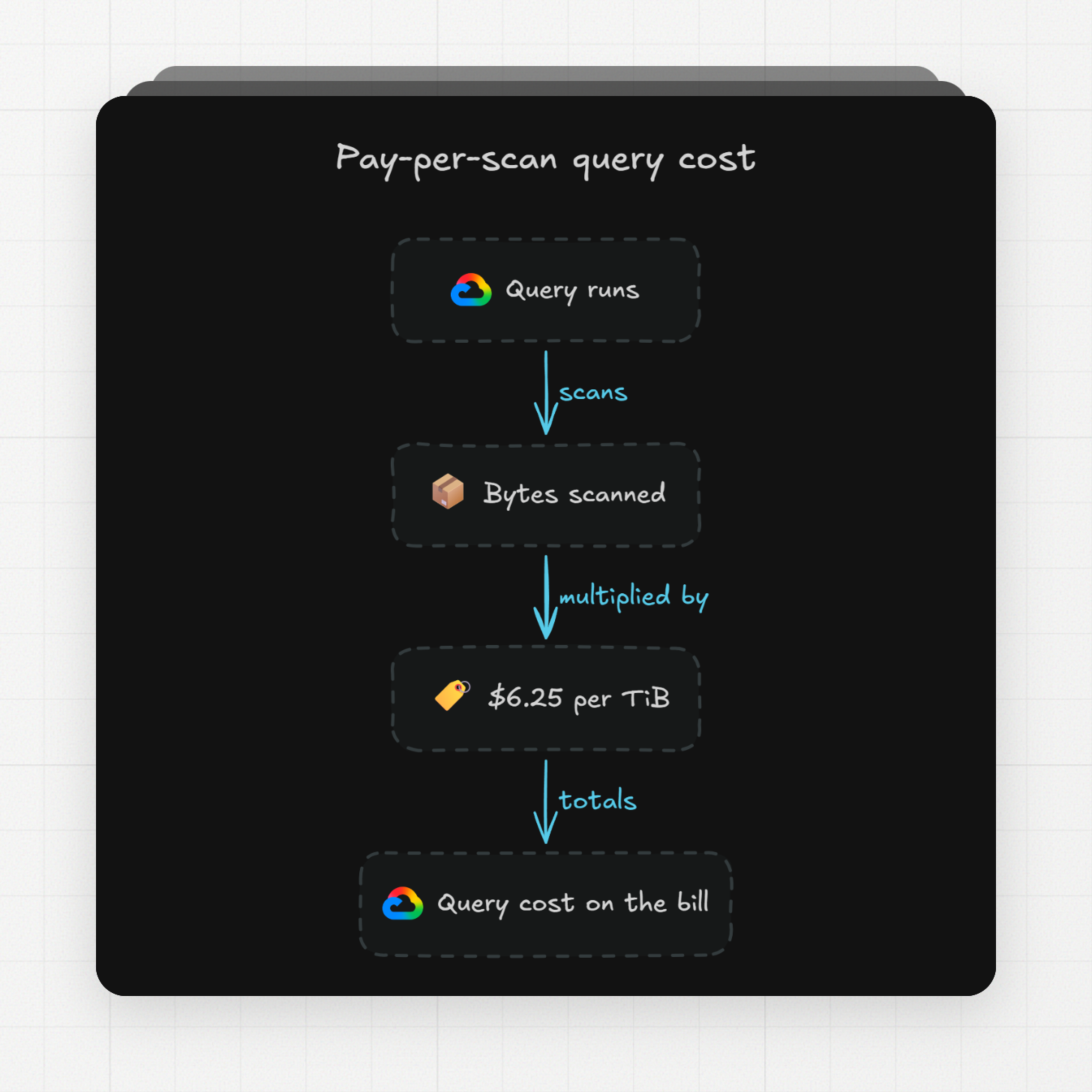
BigQuery also sells capacity for teams that prefer predictable bills: slots at $0.04 per slot-hour on the Standard edition, $0.06 on Enterprise, and $0.10 on Enterprise Plus.

The pricing model turns warehouse table design into a cost lever. The partitioning and clustering choices above, plus selecting only the columns you need instead of SELECT *, are the main tools. We cover the specific tactics in our guide to BigQuery cost optimization.

How do CDC and ELT move data from OLTP to OLAP?

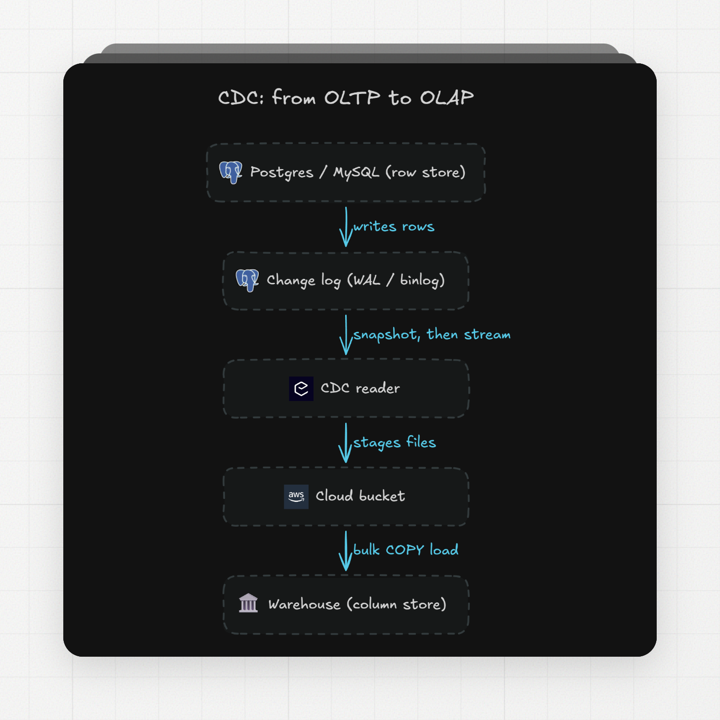
ELT (extract, load, transform) copies raw data from the transactional database into the warehouse and does the reshaping there. CDC (change data capture) is the extraction method that reads the database's own change log instead of querying tables, so every insert, update, and delete arrives in order without loading the source. The standard production pattern uses two dedicated databases connected by CDC: Postgres or MySQL take the writes, a warehouse takes the analytical reads, and a pipeline copies between them.

The change log already exists. Postgres writes every change to the write-ahead log (WAL) before applying it, and MySQL writes every change to the binary log (binlog). Both databases use these logs for their own replication. A CDC pipeline connects as if it were a replica and reads the same stream. In MySQL's case, every INSERT, UPDATE, and DELETE is captured as it is written to the log, in order, with the complete row state.

The source needs a few settings turned on. For Postgres, the Erathos connector needs wal_level set to logical, at least 10 replication slots and WAL senders, and a limit on max_slot_wal_keep_size. The last setting matters because a replication slot keeps WAL files around until the reader consumes them, with no limit by default, so a stalled pipeline can fill the disk. The docs' example sets a 5 GB ceiling. For MySQL, the binlog must be in ROW format with FULL row images, and the replication user needs SELECT, RELOAD, SHOW DATABASES, REPLICATION SLAVE, and REPLICATION CLIENT privileges.

A CDC pipeline runs in two phases. In Erathos, the snapshot mode called initial takes a full copy of the tables first and then streams changes from the log. The mode called no_data skips the copy and streams only the changes available in the log. Erathos stages the extracted data in a cloud bucket, loads it into the warehouse with COPY or the destination's equivalent bulk command, and deletes the temporary files when the job finishes. Bulk loading is the write pattern a columnar warehouse is built for, which is why CDC and OLAP fit together.

CDC is one of three ways to load a table. Erathos also offers Full Refresh, which overwrites the destination table on each run, and Partial syncs, which pick up rows past a cursor such as updated_at. Partial syncs need a primary key and a date or datetime column to use as the cursor. Full Refresh is simple and fine for small lookup tables. Partial syncs are cheap but cannot see deletes. CDC catches everything, including deletes and intermediate states, at the cost of the source configuration above.

Can one database handle both OLTP and OLAP?

Some databases try, under the name HTAP (hybrid transactional/analytical processing). They work by keeping two copies of the data, one in row format and one in column format, inside one system. The tradeoffs of each layout do not disappear. The system manages them for you within limits the vendors document.

TiDB is the clearest example. It runs a row-based storage engine, TiKV, for OLTP and a columnar engine, TiFlash, for OLAP, which replicate data automatically with strong consistency. TiDB's own guidance scopes where one database replaces a full stack: data under 100 TB and analytical concurrency under 10. It also notes that when write throughput passes 10 million rows per hour, the replication traffic between the two engines becomes a bottleneck.

AlloyDB, Google's Postgres-compatible service, takes a lighter approach. Its columnar engine keeps an in-memory column copy of selected tables and uses it to speed up scans, joins, and aggregates. By default it takes 30% of the instance's memory. Frequent updates to rows invalidate the columnar data, and for tables under about 5,000 rows the planner may use the row store anyway.

HTAP fits a mid-sized system with a small number of analysts who want fresh numbers without a pipeline. Once the analytics side grows, the data grows past what an in-memory column copy can hold, or more than a handful of people run heavy queries at once, the two-system pattern with CDC in between is the one that scales, and it is the one the warehouses themselves are built around.

FAQ

Is PostgreSQL an OLAP or OLTP database?

PostgreSQL is an OLTP database. It stores rows together, indexes them with B-trees, and is built for many small transactions per second. Extensions and managed variants such as AlloyDB's columnar engine can speed up some analytical queries on it, but they work within the limits above (memory-bound column copies, invalidated by frequent updates). For analytics over terabytes of history, Postgres is the source that feeds a warehouse, and its WAL is what a CDC pipeline reads.

Is Snowflake OLAP or OLTP?

Snowflake is an OLAP warehouse. It stores data in columnar micro-partitions of 50 to 500 MB and prunes them by per-column metadata. A single-row UPDATE rewrites the whole micro-partition that holds the row, which is why it is loaded in bulk from an OLTP source rather than written to by an application.

Is SQL Server OLAP or OLTP?

SQL Server is an OLTP database in the standard split, alongside Postgres, MySQL, and Oracle. OLTP and OLAP describe the workload and the storage layout, not the query language. All the systems in this article accept SQL. What differs is whether the engine stores rows or columns and whether it is tuned for millisecond single-row work or for scanning millions of rows.

What is OLAP and OLTP in ETL?

In an ETL or ELT pipeline, the OLTP database is the source and the OLAP warehouse is the destination. The pipeline extracts from the transactional system (by CDC, a cursor-based partial sync, or a full refresh), loads into the warehouse, and transforms there. The separation exists so that analytical scans happen on a columnar copy and never compete with the application for the production database.

What are 5 differences between OLTP and OLAP?

1. Workload: OLTP runs the application's transactions; OLAP answers questions over history.
2. Query shape: OLTP reads or changes one row by key; OLAP filters, groups, and sums across millions of rows.
3. Storage layout: OLTP stores rows together with B-tree indexes; OLAP stores columns together and prunes partitions and blocks.
4. Schema: OLTP is normalized to avoid duplication; OLAP uses star schemas or wide tables to avoid joins.
5. Pricing: OLTP bills for provisioned instance hours; OLAP bills for bytes scanned or compute time, so table design changes the bill.

Move your production data into a warehouse

If your reporting queries still run against Postgres or MySQL, Erathos copies those tables into BigQuery, Redshift, or Databricks with CDC, partial syncs, or full refreshes, and handles the snapshot, log reading, staging, and bulk loading described above. Try Erathos free for 14 days and connect your first source in an afternoon.