How to Organize Your Data So Queries Stop Costing You a Fortune
Partitioning and clustering in BigQuery reduce the amount of data scanned per query — and the cost along with it. A guide with SQL, materialized views, and spend monitoring.
Here's the blog post translated to English:
If you've ever opened a query in BigQuery and been startled by the cost preview before even running it — or received an end-of-month bill far larger than expected — you know the price of poor data modeling. Partitioning, clustering, views, and materialized views aren't just technical details: they're the difference between pipelines that cost pennies and pipelines that silently drain your budget.
In this guide, we'll explore how each of these techniques works, when to apply them, and how to combine them to build a data warehouse that delivers real performance — without blowing the company credit card.
Partitioning: Divide and Conquer
Partitioning is an optimization technique that involves physically dividing a large table into smaller, more manageable segments called partitions. This division is based on the values of one or more columns in the table, typically date/time columns or integer identifiers [1].
How Does It Work?
When a table is partitioned, data is organized into separate storage blocks, where each block corresponds to a specific partition. For example, a sales table can be partitioned by date, with each day, month, or year stored in a distinct partition. When a query is executed with a filter on the partition column, the database system can scan only the relevant partitions, ignoring the rest. This process, known as pruning, significantly reduces the amount of data to be read, resulting in faster queries and lower operational costs [1].
Benefits of Partitioning
Improved Query Performance: By reducing the volume of data to be scanned, queries that use filters on partition columns run much faster.
Cost Reduction: Many cloud-based data warehouses, such as Google BigQuery, charge based on the amount of data processed. Partitioning minimizes this amount, directly impacting costs [1].
Simplified Management: Facilitates table maintenance by allowing operations such as deleting or expiring data at the partition level without affecting the rest of the table. This is particularly useful for data retention policies [1].
Query Cost Estimation: In systems like BigQuery, partitioning enables more accurate cost estimation before query execution, as the system can determine which partitions will be scanned [1].
Common Types of Partitioning
Partitioning types vary across platforms, but the most common include:
Time Column Partitioning: Based on DATE, TIMESTAMP, or DATETIME columns. Data is automatically allocated into hourly, daily, monthly, or yearly partitions. Example: PARTITION BY DATE(timestamp_col).
Ingestion-Time Partitioning: The system automatically assigns data to partitions based on when it is ingested. A pseudo-column (e.g., _PARTITIONTIME in BigQuery) is used for this purpose.
Integer Range Partitioning: Based on an INTEGER column, where partitions are defined by value ranges. Example: PARTITION BY RANGE_BUCKET(customer_id, GENERATE_ARRAY(0, 1000000, 10000)).
Code Example (BigQuery SQL)
To create a date-partitioned table in BigQuery:
CREATE TABLE `your_project.your_dataset.partitioned_sales_table`
(
    id STRING,
    product STRING,
    value NUMERIC,
    sale_date DATE
)
PARTITION BY sale_date
OPTIONS(
    description="Sales table partitioned by date"
)
To query data from a specific partition, the WHERE clause is used to filter by the partition column:
SELECT
    product,
    SUM(value) as total_sales
FROM
    `your_project.your_dataset.partitioned_sales_table`
WHERE
    sale_date = '2023-01-15'
GROUP BY
This example demonstrates how partitioning allows BigQuery to scan only the partition corresponding to '2023-01-15', optimizing the query. [1]
Clustering: Organizing Data to Accelerate Queries
While partitioning divides a table into physical segments, clustering organizes data within those partitions (or the entire table, if not partitioned) based on specific user-defined columns [2]. Think of partitioning as creating drawers in a cabinet, and clustering as organizing the items inside each drawer in a logical order.
How Does It Work?
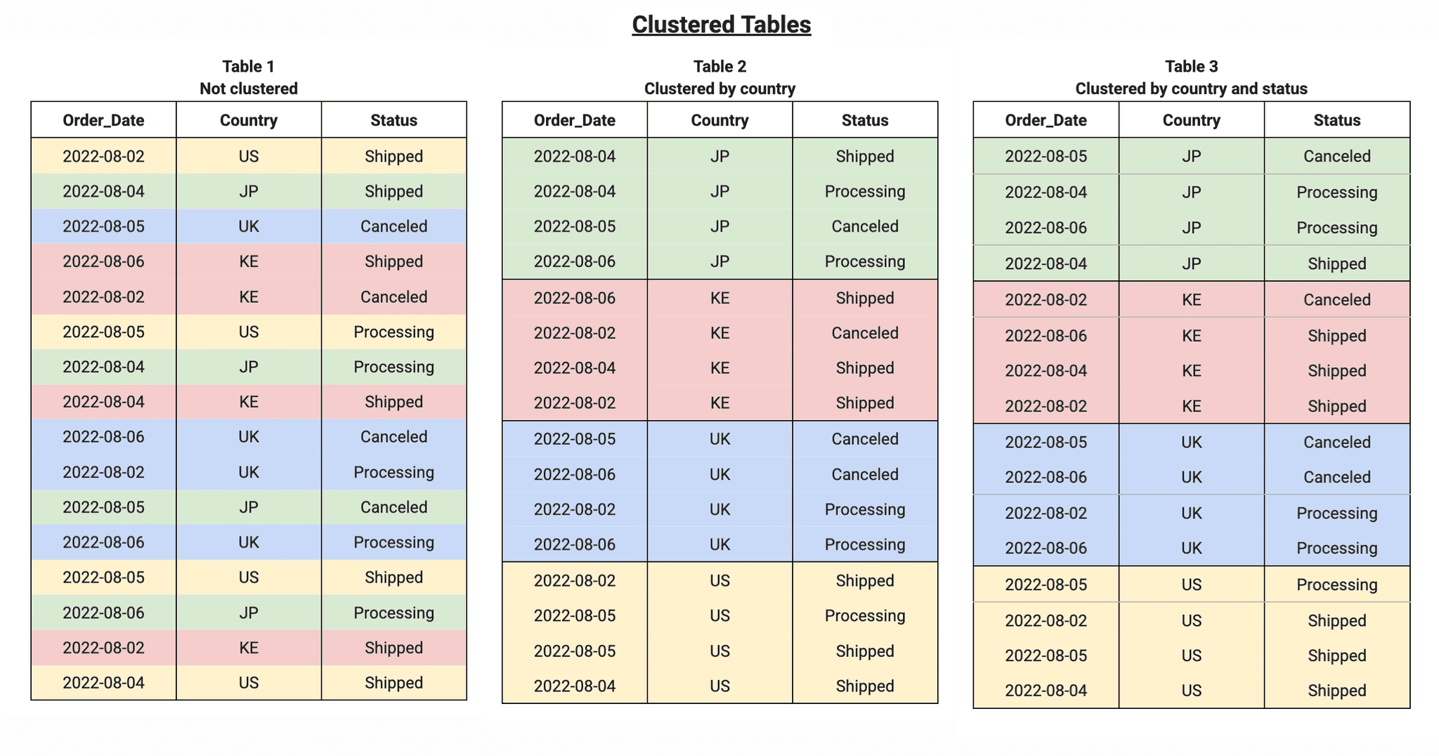
Clustering works by sorting data storage blocks based on the values of the clustered columns. When a query filters or aggregates data by those columns, the database system can scan only the relevant blocks instead of the entire partition or table. This is particularly effective for columns with high cardinality (many distinct values) [2].
For example, if a transactions table is clustered by the customer_id column, all transactions from the same customer will be stored physically close together. A query looking for transactions from a specific customer_id will benefit enormously, as the system will only need to read a small portion of the data.
Benefits of Clustering
Improved Performance on Filters and Aggregations: Speeds up queries that filter or aggregate data on clustered columns, especially those with high cardinality.
Reduced Data Scanned: Similar to partitioning, clustering allows the system to skip irrelevant data blocks, decreasing the amount of data processed and, consequently, costs [2].
Optimization for Multiple Columns: It's possible to cluster by multiple columns, and the order of those columns matters. The system optimizes searches from left to right, prioritizing the first clustered column [2].
When to Use Clustering?
Fine Granularity: When partitioning doesn't provide the granularity needed to optimize specific queries.
Filters on High-Cardinality Columns: Ideal for columns with many distinct values, where partitioning would be impractical or inefficient.
Queries with Multiple Filters or Aggregations: When queries frequently use filters or aggregations on multiple columns [2].
Large Tables or Partitions: Tables or partitions larger than 64 MB generally benefit from clustering [2].
Combining Partitioning and Clustering
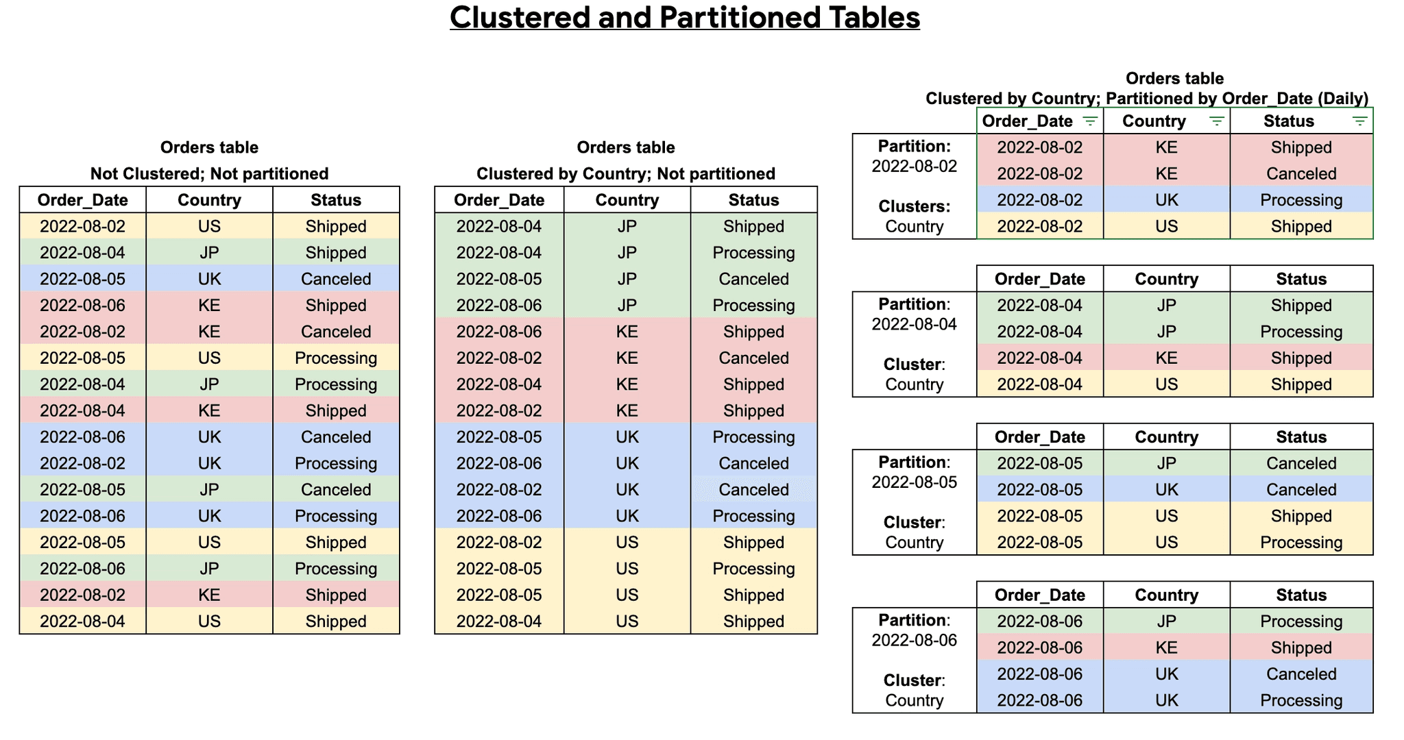
Combining partitioning and clustering is a powerful performance optimization strategy. First, the table is divided into partitions (e.g., by date), and then, within each partition, data is clustered by one or more columns (e.g., customer_id or product_category). This provides two-layer optimization, resulting in even better query performance [2].
Code Example (BigQuery SQL)
To create a table partitioned by date and clustered by product and id in BigQuery:
CREATE TABLE `your_project.your_dataset.sales_table_part_clustered`
(
    id STRING,
    product STRING,
    value NUMERIC,
    sale_date DATE
)
PARTITION BY sale_date
CLUSTER BY product, id
OPTIONS(
    description="Sales table partitioned by date and clustered by product and id"
)
In this example, data is first divided by sale_date, and within each date partition, it is organized by product and then by id. A query filtering by sale_date and product will be highly optimized. [2]
Tables, Views, and Materialized Views: What's the Difference?
Beyond optimizing physical storage with partitioning and clustering, data modeling also involves choosing the right logical structure to expose and consume that data. The three main options are Tables, Views, and Materialized Views.
1. Tables
Tables are the fundamental storage structure in any relational database or data warehouse. They store data physically on disk.
Characteristics: Data is physically persisted. DML operations (Insert, Update, Delete) modify data directly in the table.
Performance: Read performance depends on how the table is structured (indexes, partitioning, clustering).
Cost: You pay for the physical storage of data and for the processing of queries run against it.
When to use: To store the raw or processed data that forms the foundation of your data warehouse.
2. Views (Logical Views)
A View is essentially a saved SQL query that acts as a virtual table. It doesn't store data physically; instead, the underlying query is executed every time the View is queried [3].
Characteristics: Takes up no storage space (beyond the query definition). Always returns the most up-to-date data from the underlying table(s).
Performance: Performance depends entirely on the complexity of the underlying query and the volume of data in the base tables at execution time. Complex queries on Views can be slow.
Cost: You only pay for query processing every time the View is accessed.
When to use:
To simplify complex queries (encapsulating joins and aggregations).
To restrict access to specific columns or rows of a base table (security).
To create a logical abstraction layer over the physical model.
View Creation Example:
CREATE VIEW `your_project.your_dataset.daily_sales_view` AS
SELECT
    sale_date,
    SUM(value) as total_sales,
    COUNT(id) as transaction_count
FROM
    `your_project.your_dataset.partitioned_sales_table`
GROUP BY
3. Materialized Views
Materialized Views combine characteristics of both Tables and Views. They are defined by a SQL query (like a View), but the result of that query is pre-computed and physically stored on disk (like a Table) [4].
Characteristics: Store data physically. They need to be "refreshed" to reflect changes in the base tables. The refresh can be manual, scheduled, or automatic (incremental), depending on the database.
Performance: Offer extremely fast read performance since the data is already pre-computed (especially useful for heavy aggregations).
Cost: You pay for the storage of pre-computed data, for the processing required to refresh the Materialized View, and for queries run against it (which are generally much cheaper than querying the base tables).
When to use:
For dashboards and reports that require millisecond response times.
When the same complex aggregation is repeatedly queried by multiple users or processes.
When data latency (slightly outdated data between refresh cycles) is acceptable [4].
Materialized View Creation Example (BigQuery):
CREATE MATERIALIZED VIEW `your_project.your_dataset.mv_monthly_sales` AS
SELECT
    EXTRACT(MONTH FROM sale_date) as month,
    EXTRACT(YEAR FROM sale_date) as year,
    SUM(value) as total_sales
FROM
    `your_project.your_dataset.partitioned_sales_table`
GROUP BY
    month, year
Comparison Summary
Feature | Table | View | Materialized View |
|---|---|---|---|
Storage | Physical | Logical (Query Only) | Physical (Pre-computed) |
Data Freshness | Updated via DML | Always real-time | Depends on refresh frequency |
Read Performance | High (if optimized) | Depends on base query | Very High |
Costs Involved | Storage + Query | Query only | Storage + Refresh + Query (cheaper) |
Conclusion
Modern data modeling requires a deep understanding of how data is stored and accessed. Partitioning and clustering are indispensable tools for physically organizing large volumes of data, reducing costs and accelerating queries by minimizing unnecessary data reads.
On the other hand, choosing between Tables, Views, and Materialized Views defines the logical architecture of your data warehouse. While Tables hold the absolute truth, Views offer flexibility and security, and Materialized Views deliver the extreme performance needed for large-scale analytics.
Mastering these techniques is half the battle. The other half is ensuring data reaches these structures reliably — no surprises, no black boxes, no endless maintenance. That's exactly what Erathos solves.
Explore the platform →
References
[1] Google Cloud. "Introduction to partitioned tables". Available at: https://cloud.google.com/bigquery/docs/partitioned-tables
[2] Google Cloud. "Introduction to clustered tables". Available at: https://cloud.google.com/bigquery/docs/clustered-tables
[3] Databricks. "Tables and views in Databricks". Available at: https://docs.databricks.com/aws/en/data-engineering/tables-views
[4] Snowflake. "Working with Materialized Views". Available at: https://docs.snowflake.com/en/user-guide/views-materialized
Here's the blog post translated to English:
If you've ever opened a query in BigQuery and been startled by the cost preview before even running it — or received an end-of-month bill far larger than expected — you know the price of poor data modeling. Partitioning, clustering, views, and materialized views aren't just technical details: they're the difference between pipelines that cost pennies and pipelines that silently drain your budget.
In this guide, we'll explore how each of these techniques works, when to apply them, and how to combine them to build a data warehouse that delivers real performance — without blowing the company credit card.
Partitioning: Divide and Conquer
Partitioning is an optimization technique that involves physically dividing a large table into smaller, more manageable segments called partitions. This division is based on the values of one or more columns in the table, typically date/time columns or integer identifiers [1].
How Does It Work?
When a table is partitioned, data is organized into separate storage blocks, where each block corresponds to a specific partition. For example, a sales table can be partitioned by date, with each day, month, or year stored in a distinct partition. When a query is executed with a filter on the partition column, the database system can scan only the relevant partitions, ignoring the rest. This process, known as pruning, significantly reduces the amount of data to be read, resulting in faster queries and lower operational costs [1].
Benefits of Partitioning
Improved Query Performance: By reducing the volume of data to be scanned, queries that use filters on partition columns run much faster.
Cost Reduction: Many cloud-based data warehouses, such as Google BigQuery, charge based on the amount of data processed. Partitioning minimizes this amount, directly impacting costs [1].
Simplified Management: Facilitates table maintenance by allowing operations such as deleting or expiring data at the partition level without affecting the rest of the table. This is particularly useful for data retention policies [1].
Query Cost Estimation: In systems like BigQuery, partitioning enables more accurate cost estimation before query execution, as the system can determine which partitions will be scanned [1].
Common Types of Partitioning
Partitioning types vary across platforms, but the most common include:
Time Column Partitioning: Based on DATE, TIMESTAMP, or DATETIME columns. Data is automatically allocated into hourly, daily, monthly, or yearly partitions. Example: PARTITION BY DATE(timestamp_col).
Ingestion-Time Partitioning: The system automatically assigns data to partitions based on when it is ingested. A pseudo-column (e.g., _PARTITIONTIME in BigQuery) is used for this purpose.
Integer Range Partitioning: Based on an INTEGER column, where partitions are defined by value ranges. Example: PARTITION BY RANGE_BUCKET(customer_id, GENERATE_ARRAY(0, 1000000, 10000)).
Code Example (BigQuery SQL)
To create a date-partitioned table in BigQuery:
CREATE TABLE `your_project.your_dataset.partitioned_sales_table`
(
    id STRING,
    product STRING,
    value NUMERIC,
    sale_date DATE
)
PARTITION BY sale_date
OPTIONS(
    description="Sales table partitioned by date"
)
To query data from a specific partition, the WHERE clause is used to filter by the partition column:
SELECT
    product,
    SUM(value) as total_sales
FROM
    `your_project.your_dataset.partitioned_sales_table`
WHERE
    sale_date = '2023-01-15'
GROUP BY
This example demonstrates how partitioning allows BigQuery to scan only the partition corresponding to '2023-01-15', optimizing the query. [1]
Clustering: Organizing Data to Accelerate Queries
While partitioning divides a table into physical segments, clustering organizes data within those partitions (or the entire table, if not partitioned) based on specific user-defined columns [2]. Think of partitioning as creating drawers in a cabinet, and clustering as organizing the items inside each drawer in a logical order.
How Does It Work?
Clustering works by sorting data storage blocks based on the values of the clustered columns. When a query filters or aggregates data by those columns, the database system can scan only the relevant blocks instead of the entire partition or table. This is particularly effective for columns with high cardinality (many distinct values) [2].
For example, if a transactions table is clustered by the customer_id column, all transactions from the same customer will be stored physically close together. A query looking for transactions from a specific customer_id will benefit enormously, as the system will only need to read a small portion of the data.
Benefits of Clustering
Improved Performance on Filters and Aggregations: Speeds up queries that filter or aggregate data on clustered columns, especially those with high cardinality.
Reduced Data Scanned: Similar to partitioning, clustering allows the system to skip irrelevant data blocks, decreasing the amount of data processed and, consequently, costs [2].
Optimization for Multiple Columns: It's possible to cluster by multiple columns, and the order of those columns matters. The system optimizes searches from left to right, prioritizing the first clustered column [2].
When to Use Clustering?
Fine Granularity: When partitioning doesn't provide the granularity needed to optimize specific queries.
Filters on High-Cardinality Columns: Ideal for columns with many distinct values, where partitioning would be impractical or inefficient.
Queries with Multiple Filters or Aggregations: When queries frequently use filters or aggregations on multiple columns [2].
Large Tables or Partitions: Tables or partitions larger than 64 MB generally benefit from clustering [2].
Combining Partitioning and Clustering
Combining partitioning and clustering is a powerful performance optimization strategy. First, the table is divided into partitions (e.g., by date), and then, within each partition, data is clustered by one or more columns (e.g., customer_id or product_category). This provides two-layer optimization, resulting in even better query performance [2].
Code Example (BigQuery SQL)
To create a table partitioned by date and clustered by product and id in BigQuery:
CREATE TABLE `your_project.your_dataset.sales_table_part_clustered`
(
    id STRING,
    product STRING,
    value NUMERIC,
    sale_date DATE
)
PARTITION BY sale_date
CLUSTER BY product, id
OPTIONS(
    description="Sales table partitioned by date and clustered by product and id"
)
In this example, data is first divided by sale_date, and within each date partition, it is organized by product and then by id. A query filtering by sale_date and product will be highly optimized. [2]
Tables, Views, and Materialized Views: What's the Difference?
Beyond optimizing physical storage with partitioning and clustering, data modeling also involves choosing the right logical structure to expose and consume that data. The three main options are Tables, Views, and Materialized Views.
1. Tables
Tables are the fundamental storage structure in any relational database or data warehouse. They store data physically on disk.
Characteristics: Data is physically persisted. DML operations (Insert, Update, Delete) modify data directly in the table.
Performance: Read performance depends on how the table is structured (indexes, partitioning, clustering).
Cost: You pay for the physical storage of data and for the processing of queries run against it.
When to use: To store the raw or processed data that forms the foundation of your data warehouse.
2. Views (Logical Views)
A View is essentially a saved SQL query that acts as a virtual table. It doesn't store data physically; instead, the underlying query is executed every time the View is queried [3].
Characteristics: Takes up no storage space (beyond the query definition). Always returns the most up-to-date data from the underlying table(s).
Performance: Performance depends entirely on the complexity of the underlying query and the volume of data in the base tables at execution time. Complex queries on Views can be slow.
Cost: You only pay for query processing every time the View is accessed.
When to use:
To simplify complex queries (encapsulating joins and aggregations).
To restrict access to specific columns or rows of a base table (security).
To create a logical abstraction layer over the physical model.
View Creation Example:
CREATE VIEW `your_project.your_dataset.daily_sales_view` AS
SELECT
    sale_date,
    SUM(value) as total_sales,
    COUNT(id) as transaction_count
FROM
    `your_project.your_dataset.partitioned_sales_table`
GROUP BY
3. Materialized Views
Materialized Views combine characteristics of both Tables and Views. They are defined by a SQL query (like a View), but the result of that query is pre-computed and physically stored on disk (like a Table) [4].
Characteristics: Store data physically. They need to be "refreshed" to reflect changes in the base tables. The refresh can be manual, scheduled, or automatic (incremental), depending on the database.
Performance: Offer extremely fast read performance since the data is already pre-computed (especially useful for heavy aggregations).
Cost: You pay for the storage of pre-computed data, for the processing required to refresh the Materialized View, and for queries run against it (which are generally much cheaper than querying the base tables).
When to use:
For dashboards and reports that require millisecond response times.
When the same complex aggregation is repeatedly queried by multiple users or processes.
When data latency (slightly outdated data between refresh cycles) is acceptable [4].
Materialized View Creation Example (BigQuery):
CREATE MATERIALIZED VIEW `your_project.your_dataset.mv_monthly_sales` AS
SELECT
    EXTRACT(MONTH FROM sale_date) as month,
    EXTRACT(YEAR FROM sale_date) as year,
    SUM(value) as total_sales
FROM
    `your_project.your_dataset.partitioned_sales_table`
GROUP BY
    month, year
Comparison Summary
Feature | Table | View | Materialized View |
|---|---|---|---|
Storage | Physical | Logical (Query Only) | Physical (Pre-computed) |
Data Freshness | Updated via DML | Always real-time | Depends on refresh frequency |
Read Performance | High (if optimized) | Depends on base query | Very High |
Costs Involved | Storage + Query | Query only | Storage + Refresh + Query (cheaper) |
Conclusion
Modern data modeling requires a deep understanding of how data is stored and accessed. Partitioning and clustering are indispensable tools for physically organizing large volumes of data, reducing costs and accelerating queries by minimizing unnecessary data reads.
On the other hand, choosing between Tables, Views, and Materialized Views defines the logical architecture of your data warehouse. While Tables hold the absolute truth, Views offer flexibility and security, and Materialized Views deliver the extreme performance needed for large-scale analytics.
Mastering these techniques is half the battle. The other half is ensuring data reaches these structures reliably — no surprises, no black boxes, no endless maintenance. That's exactly what Erathos solves.
Explore the platform →
References
[1] Google Cloud. "Introduction to partitioned tables". Available at: https://cloud.google.com/bigquery/docs/partitioned-tables
[2] Google Cloud. "Introduction to clustered tables". Available at: https://cloud.google.com/bigquery/docs/clustered-tables
[3] Databricks. "Tables and views in Databricks". Available at: https://docs.databricks.com/aws/en/data-engineering/tables-views
[4] Snowflake. "Working with Materialized Views". Available at: https://docs.snowflake.com/en/user-guide/views-materialized